When disaster strikes, we tend to focus on the storm, the flood, or the earthquake itself. But after two decades of fieldwork across Southeast Asia and Japan, I keep coming back to something less visible — and just as powerful: the culture, institutions, and social structures of the communities involved shape survival just as much as the disaster itself.
It’s Not Just About the Disaster
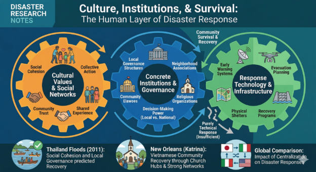
Sociologist Benjamin F. McLuckie compared disaster responses across Japan, Italy, and the United States as far back as the 1970s. His key finding: how centralized a government is — how much decision-making power sits with national versus local authorities — significantly shapes what actually happens on the ground when emergencies unfold.
But culture alone does not explain everything. What really drives outcomes is a three-way mix of culture, institutions, and technology. A community that values collective action still needs neighborhood associations, shelters, and early warning systems to turn that value into real protection. Without those structures, values remain just values.
What I Found in the Field
My work on the 2011 Thailand floods — which disrupted global supply chains and devastated communities around industrial parks — brought this home clearly. Social cohesion and local governance structures were just as predictive of recovery as physical flood barriers. Through the Japan-Thailand SATREPS collaboration, my colleagues and I developed community capacity assessments and social vulnerability indices to help local leaders act before the next disaster, not scramble after it.
What struck me most was this: communities with strong internal networks recovered faster, not because they had more resources, but because they already knew how to work together.
The New Orleans Lesson
After Hurricane Katrina in 2005, researchers noticed that Vietnamese-American communities in New Orleans recovered more quickly than many others. The easy explanation was “culture.” But the real answer was more grounded: strong churches functioning as organizing hubs, dense social networks built through shared migration experience, and established community leadership capable of coordinating a return. Culture mattered — but it worked through concrete institutions. That distinction is important.
Why This Matters Now
Climate change is making disasters more frequent and more severe. Yet many governments still treat disaster response as a purely technical problem — better seawalls, faster alert systems. Those matters. But they miss the human layer that makes those tools actually work.
When we recognize that community trust, family networks, and local governance are all part of the disaster equation, we can design better evacuation plans, more effective early warnings, and recovery programs that genuinely reach the people who need them most.
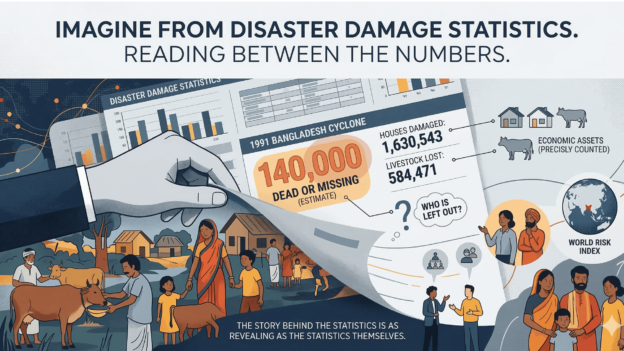
Every disaster holds up a mirror to the society it strikes. What we see reflected — who gets help quickly, who rebuilds together, who gets left behind — is shaped by culture, institutions, and history working in combination. That is not just a scholarly observation. It is, ultimately, a matter of life and death.
Sources:
McLuckie, B.F. (1977). Italy, Japan, and the United States: Effects of Centralization on Disaster Responses. University of Delaware;
Nakasu, T. et al. (2022). International Journal of Disaster Resilience and Built Environment. https://doi.org/10.1108/IJDRBE-10-2020-0107;
Nakasu, T. (2023). Environmental Development and Sustainability. https://doi.org/10.1007/s10668-023-04305-7